Going forward, going back: how all neural networks learn

💫 We open a neural network and see how it learns; we talk about the loss and backpropagation; Paris celebrates Fête de la musique

Jun 23, 2024

Last week we trained a language-generating neural network on the complete works of Shakespeare. At the beginning, the output didn’t look like English sentences at all:

wiry hurts mourns met hizzing craftily playfellow be beaks conditions is applauding easiest tiddle dismissing pieces jenny

but after a few cycles it got better:

romeo be heard and this mighty ears twill
bawd , emperial ! ; steal it
cry heavens dost successful i say
children scattering , sir

What we didn’t explain yet is how exactly the network learned to improve its results. Let’s look at this question today and introduce the key technique that unlocked all of the AI innovation we see today: backpropagation.

Going forward

Neural networks are first initialized with random values and then trained on examples.

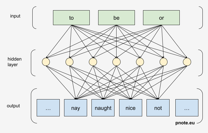
Our neural network uses three words of context at a time and learns to predict the fourth word. Training examples for this problem derived from the famous sentence “To be or not to be” could look like this:

[❌, ❌, ‘to’] → ‘be’
[❌, ‘to’, ‘be’] → ‘or’
[‘to’, ‘be’, ‘or’] → ‘not’
… etc.

These training examples are run through the network. For example, we’d set the input of the network to [‘to’, ‘be’, ‘or’] , and then calculate its prediction of the next word.

At this stage, the calculations are done top-to-bottom. The weights stored in the arrows are multiplied by the input numbers. At the end we get a probability distribution of what the network thinks are the next likely words.

What a loss

Once we get the network prediction, we compare it to the correct result from the training data set. Specifically, we calculate how far we are from the right answer. This measure of how far we are is called a “loss”.

On the example of [‘to’, ‘be’, ‘or’] → ‘not’ , the right next word is “not”. We’d look at the network prediction and …

… if the network predicted “not” as 100% probable, we’re exactly on target and we’d calculate the loss as 0.0
… if the network predicted “not” as 75% probable, the loss would be a small number, for example 0.13
... if the network predicted “not” as 0.01% probable (almost impossible), we’d assign a very high loss, for example 12.23

⭐️ Loss. A measure of how far a neural network prediction is from the correct output. (The lower the loss the better.)

Going backwards

The final ingredient of the algorithm is the most important one. We start with the resulting loss at the bottom of the network, and then go through all the computations in reverse (bottom-to-top). At each node:

if the resulting value was too big, we nudge its inputs to make the result a bit smaller the next time
if the resulting value was too small, we nudge its inputs to make the result a bit bigger the next time

⭐️ Backpropagation. Going backward through the neural network computation graph and adjusting the weights to make the resulting loss smaller.

Conclusion

This is what it means in practice: whenever we build a neural network, we design the architecture and we select the loss function.

The loss function is the formula that we use to guide the adjustments we make to the neural network weights during training. Without the loss function, we cannot train.

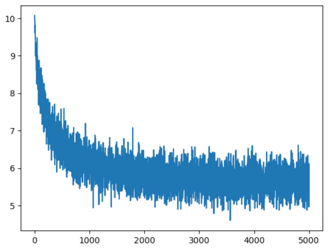
When the model trains well, we see the loss improving over time and eventually converging. Here’s the training chart showing loss over time for my neural net as it trained on the complete works of Shakespeare:

Yes, it’s expected that the chart looks so jagged. This is because each time we run the network only on a handful of examples, so there will be a lot of noise / variation in how accurate the network is on each batch.

In other news

🤖 LLM of the week: Claude 3.5 Sonnet. The new model from Anthropic comes with state-of-the art performance and new output modalities. The Verge calls Claude’s naming scheme (Haiku, Sonnet, Opus) weird but I love it 🫶.
🔧 Semianalysis note on the scale of big GPU clusters: Multiple large AI labs including but not limited to OpenAI/Microsoft, xAI, and Meta are in a race to build GPU clusters with over 100,000 GPUs. These individual training clusters cost in excess of $4 billion of server capital expenditures alone (…). A 100,000 GPU cluster will require >150MW in datacenter capacity and guzzle down 1.59 terawatt hours in a single year, costing $123.9 million at a standard rate of $0.078/kWh.
💫 Meanwhile, Ilya Sutskever, one of OpenAI’s co-founders, launches a new company called Safe Superintelligence. History will tell how many big LLMs can be sustained by the market, given the high training costs (see above).

Postcard from Paris

France celebrates the summer solstice with the annual fête de la musique .

I still believe
In the need
For guitars and drums and desperate poetry
(I still believe – Frank Turner)

Have a great week 🎵
– Przemek

pnote

Discussion about this post